Notes

How can we quantitatively characterize renewable output intermittency?

26 August 2026 /6 min read

How the problem comes up

Over the past few years, our team has been using mathematical tools to optimize the sizing of renewable hydrogen systems. In these systems, variable wind and solar output supplies electrolysis, while the downstream user usually needs a relatively stable hydrogen feed. Storage, renewable oversizing, and sometimes grid support help bridge this mismatch.

However, the sizing results are often difficult to explain intuitively. Why do two wind profiles with the same annual capacity factor lead to different optimal system sizes? Why does one require more storage and greater electrolyzer oversizing? We usually attribute this to different intermittency properties, but can seldom describe the difference precisely. Sometimes we fall into circular reasoning: a profile is more intermittent because the model requires more storage, and it requires more storage because it is more intermittent. Looking at the curves and relying on engineering intuition gives us only limited insight.

We wanted a comprehensive way to describe these differences quantitatively and discuss the output profile independently of the optimization result. A few weeks ago, I decided to give the task to GPT.

Vibe research, step by step

I fed GPT the engineering context, a few examples, and my half-formed ideas, asking for scalar or curve-based indicators to describe intermittency and help explain the sizing results. Then I sat back, hoping the magic AI would sort it all out in one go. But the response fell short of my expectations: it offered a few useful ideas, yet covered only a small part of what I was trying to understand.

I realized I needed to be a bit more patient. So I broke the work into smaller jobs and worked through them with GPT, one at a time:

Clarify the engineering problem and its scope.
Agree on what would make a useful indicator: helpful for comparing profiles, easy to interpret, and with few tunable parameters.
Cast the net wide and brainstorm candidate indicators.
Go through the candidates one by one, evaluate them against the agreed criteria and shortlist the most useful ones.

GPT came back with more than fifty candidates this time, and after a second round of review, we were down to twenty. Along the way, we settled on describing one output curve at a time, whether it came from wind, solar, or a fixed blend of the two. Choosing the wind–solar mix and calculating storage or grid support through dispatch remained separate problems. We kept our linear-programming (LP) model for validation.

A few indicator examples

Twenty indicators are a lot to take in. Let’s start with three and see what they can tell us about system sizing.

Output duration curve

Output duration curves are widely used in power engineering. By sorting hourly generation from highest to lowest, they show approximately how often output reaches or exceeds a given level. If most hours have low-to-medium output, a relatively small electrolyzer can absorb the available power during those hours. Drawing a horizontal line at its rated power makes the tradeoff visible: the area between the curve and the line, wherever generation exceeds that capacity, indicates the energy that would be curtailed if electrolysis were the only outlet.

Moving-window output quantiles

To examine weak generation over several hours or days, we calculate the $n$ -hour moving average of a record containing $T$ hourly output values $x_t$ :

m_t(n)=\frac{1}{n}\sum_{j=0}^{n-1}x_{t+j}, \qquad t=1,\ldots,T-n+1.

We then take the empirical $p$ -quantile, $Q_p$ , of these window averages:

A_p(n)=Q_p\!\left(\{m_1(n),\ldots,m_{T-n+1}(n)\}\right).

P0 ( $p=0$ ) gives the lowest window average, while P10 ( $p=0.10$ ) gives the 10th percentile. A small gap between them means roughly the lowest 10% of window averages lie close to the minimum. By varying the window length, we can see how weak average supply can be over a day, a week, or longer.

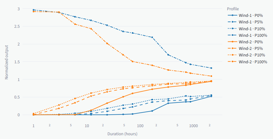
If the quantile curves cluster near the mean at window lengths well below the full record, fluctuations largely balance out over those durations, giving similar average supply across windows. If the lower quantiles remain well below the mean at weekly or longer durations, weak average generation persists over longer periods. For a steady hydrogen feed, such periods can keep drawing down hydrogen reserves, requiring more storage or sustained grid-supported electrolysis.

Maximum cumulative deficit

Maximum cumulative deficit measures the largest net energy shortfall over any continuous interval relative to a chosen reference output. Shortfalls below the reference add to the deficit, while surplus above it provides recovery. Several weak periods can therefore form one large cumulative shortfall when the intervening surplus only partly makes up the missing energy.

For a renewable hydrogen system, we can set the reference to the electrolysis power required for a steady hydrogen feed. This helps describe the combined burden of successive production shortfalls: a brief improvement in generation may provide too little recovery before the next weak period begins. The largest accumulated shortfall provides an indication of the storage capacity needed to maintain that feed.

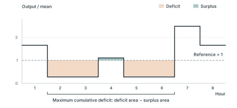
A teaching example showing a continuous deficit interval with a brief recovery inside it.

The surplus at hour 4 only partly offsets the surrounding deficits, so the largest net shortfall spans hours 2 to 6.

Building the indicator app

If you find the explanations above a bit obscure, that was also my impression when reading the documentation delivered by GPT. I thought the best way forward was to proceed directly to the next step of web app development and see how they behaved on real profiles.

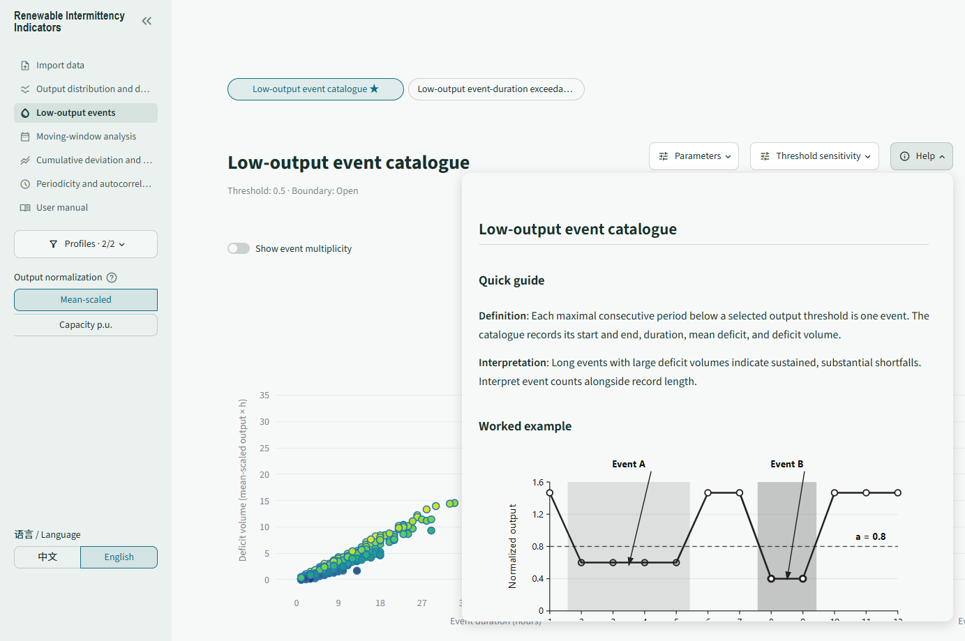
The app is now online on Streamlit Community Cloud, and you’re welcome to try it with your own wind or solar profiles. Together with GPT we also spent quite some effort on the help for each indicator. A quick guide explains what it measures, followed by formulas, notes on interpretation, and SVG illustrations that work through a small example. It serves as a detailed reference manual that helps readers understand each indicator in context.

Next steps

I am still getting familiar with some of the indicators. Trying the app on more real profiles could give a better sense of which ones add useful insight, and perhaps suggest improvements to the collection and the explanations.

A possible follow-up would be to compare the indicators with the hydrogen-system LP, using controlled and real profiles under consistent assumptions and matching average input when comparing profile shape. It would be interesting to see how these measures relate to changes in storage, electrolyzer sizing, and grid use.